Face Recognition based on CNN
Chen Yang
Department of Electrical & Computer Engineering
Hebert Wertheim College of Engineering
University of Florida
cyang3@ufl.edu
Abstract
Face recognition plays a vital role in the real-world applications, such as video surveillance, human-computer interaction, and security systems. Compared with traditional machine learning methods, the recently emerging implementations based on deep learning technology have better performance in terms of recognition speed and accuracy. This paper will implement and analyze an online face recognition system based on enhanced version of LeNet model. The main contents are basic introduction of face recognition technology, specific architecture of the CNN model, and the analysis of the system output.
Keywords —— Face recognition; Deep learning, LeNet, Convolutional neural networks (CNN)
Ⅰ.Introduction
As one of the biometric identification technology, face recognition has many unique advantages, such as low cost, non-contact, and stable verification speed, etc. In recent years, as a new research direction of machine learning technology, deep learning has made remarkable achievements in the field of image processing and computer vision applications. Among various deep learning networks, convolutional neural networks have shown extraordinary image processing capabilities because of its special structure of local weight sharing. Therefore, CNN is an extremely powerful tool to process image. In addition to face recognition, CNN has a wider range of applications, such as image classification and retrieval, target positioning and segmentation, etc.
The main contribution of this paper is to obtain a recognition algorithm with high reliability and accuracy. The general structure of face recognition process in this paper is made up of four steps. It starts with the collection of face dataset, continues with building neural networks and afterwards training the CNN model with the processed pictures, finally we can achieve real-time face recognition with the trained neural network model.
The rest parts of this paper is organized as follows. In section 2, the basic CNN structure and working characteristics will be introduced. In the section 3, the comprehensive implementation process of the proposed algorithm will be discussed. In section 4 and 5, the experimental results and some summarization based on the output will be given.
Ⅱ. Methodology
A typical convolutional neural network usually consists of the following layers: input layer, convolutional layer, Relu layer, pooling layer and fully connected layer. By overlaying these layers, a complete convolutional neural network is successfully constructed. However, in actual implementations, computer programmers often combine the convolutional layer and the ReLU layer as a convolutional layer, so the convolutional layer also needs to go through an activation function after a convolution operation. Convolutional layers and pooling layers generally appear alternately in neural network models. In other words, a pair of convolutional layer and pooling layer can be regarded as a process of feature extraction, however, not every appearance of convolutional layer is accompanied by a pooling layer. Most networks only contain three pooling layers, and end up with one or two fully connected layers.
The next paragraph is a brief introduction to the various layers in the convolutional neural networks. (This article will skip the introduction of the input layer and output layer. Their composition and function are the same as those of general artificial neural networks.)
The convolutional layer in the neural network is responsible for feature extraction of the data. The main computing process can be understood as scanning the entire picture with a convolution kernel (filter), and then obtaining the local feature values of these areas by filtering each small block of image. In practical applications, multiple convolution kernels are generally used to process images. In these kernels, each represents a kind of image pattern. If the output value of a convolution kernel corresponding to a certain image area is relatively large, it means that this area is very close to the current convolutional kernel.
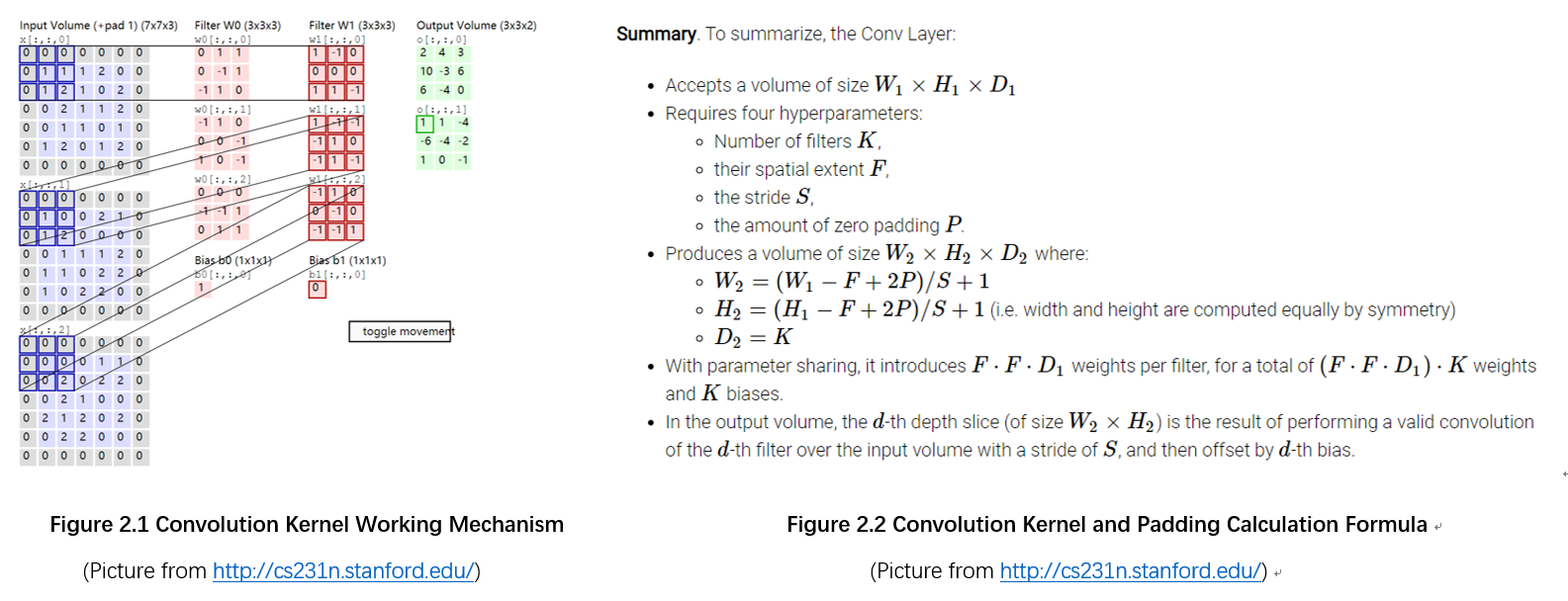
The pooling layer is responsible for dimensionality reduction of the data. Therefore, the pooling layer is generally called the downsampling layer. When the pooling layer is working, the sampling window scans the entire picture like the convolution kernel, and each movement generally retains the average or maximum value of the current area. The reason why the pooling layer is used is that after the features are extracted by the convolution kernel, the output image is still very large, so the pooling layer is used to do the demensionality reduction to reduce the total amount of data and avoid overfitting as much as possible.

The fully connected layer is responsible for receiving the data processed by the convolutional layer and the pooling layer, and then connected all the neurons with features activated in the network, finally classify and output the result.
Ⅲ. Experimental Design
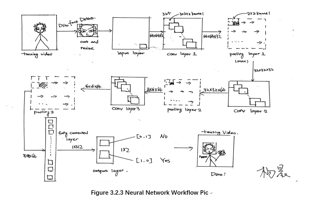
This design successfully runs on win10, the compiler is Pycharm, the main framework of neural network is implemented by tensorflow, and the python version is 3.5. The version information of other libraries called will be listed below. The entire online recognition system can be divided into four parts, of which the first three parts will be explained in detail in this chapter.
3.1 Image Prepossessing
The final task of the project is to output a successful classification network, so in this part, two kind of face data sets are required, {other_faces} and {my_faces}.
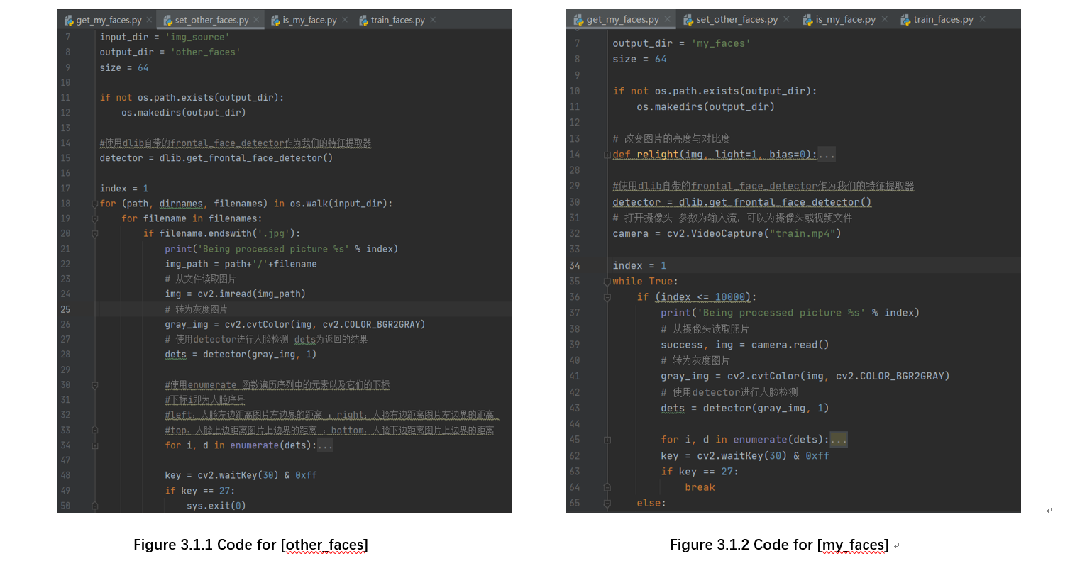
{other_faces}: The data set for this step is “Labeled Faces in the Wild Home (2019)”, downloaded from http://vis-www.cs.umass.edu/lfw/lfw.tgz . The data set contains 13,233 face images, the size of these pictures is 250×250. After the download is completed, unzip the image to the {img_source} folder. Then use dlib to batch process the images and save the output pictures to the directory {other_faces}. (dlib frontal dectector can recognize the part of the picture that contains the face and save it. After resizing, the output image size is 64×64.)
{my_faces}: The data set for this step is collected from video “training.mp4”. The position of the face is detected, the coordinates and size are returned, and the face is intercepted by the method of array slicing, and the intercepted small picture is saved as a data set. This step obtains 10,000 face data sets of oneself, and uses dlib frontal detector to recognize faces.

3.2 Analysis of Internal Structure of Neural Network
The size of the picture obtained after preprocessing is 64×64×3. Next, pass the processed pictures into the eight-layer neural network designed for this experiment. This design builds an 8-layer neural network. The detailed structure analysis and image processing process are as follows.
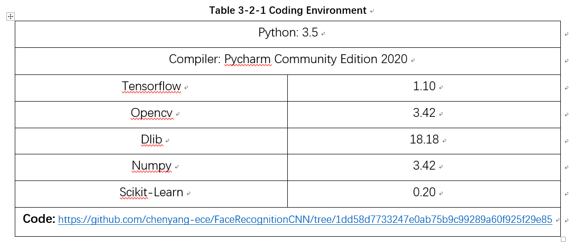
In the neural network model, the first set of layers are conv1 and pooling1. The size of the convolution kernel is 3×3. The image processed by 32 different convolution kernels are stacked as the output of conv1. The output picture enters the pooling layer. Pooling1 samples the maximum value of the current image area. The size of pooling filter is 2×2. In the whole networks, the padding size is SAME. The input of the first set of layers is 64×64×3, the output of the first set is 32×32×32.
The second set of layers are conv2 and pooling2. The size of the kernels in this set and the workflow are exactly the same as the layers in the first set. Input size: 32×32×32, Output size: 16×16×64.
Similarly, the third set (conv3 and pooling3 ) is also the same as the first two sets. Input size: 16×16×64, Output size:8×8×64.

The seventh layer of the network is a fully connected layer, whose function is to adjust the size of the output data of the previous layer from 8×8×64 to 1×4096, and then output the data after the weighted sum is calculated. The output of this layer is 1×512.
The eighth layer is also a fully connected layer, which is used to classify the output of the previous layer according to the label division in the code, and the output size is 1×2.

3.3 CNN Training
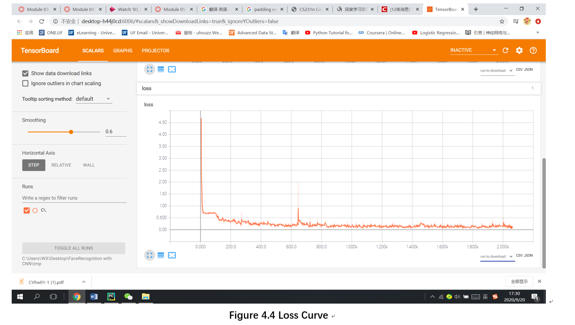
After image processing and model construction, CNN training can officially begin. According to the instruction of the lfw database website, training set and validation set are recommended to be generated by splitting the data set randomly. Therefore, we first merge the two data sets({my_faces} and {other_faces}), and then randomly divide the training set and the validation set at a ratio of 20:1. The loss function chosen in this project is cross entropy, the optimizer is Adam.
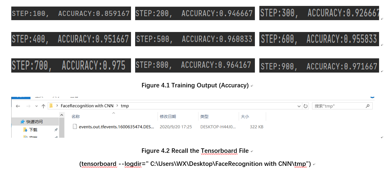
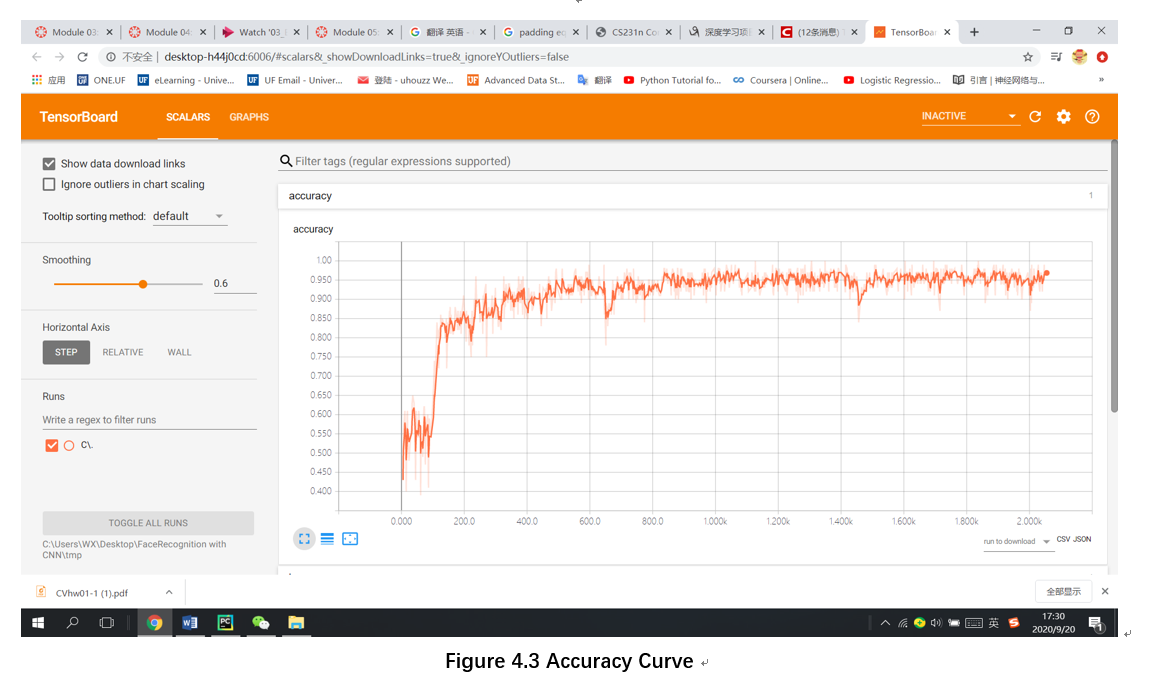
In this section, the batch size is chosen to be 100 and the learning rate = 0.01. Record the loss at each step, calculate the average accuracy every 100 steps, and save the training accuracy and loss curve as a temporary file in the directory ” \tmp”(Save it in tensorboard file format for later recall). The specific implementation code and accuracy calculation formula are shown in the figure below.

Ⅳ. Evaluation
Ⅴ. Conclusion
This design mainly studies the online face recognition system based on the improved LeNet model. In addition, it also implements video face collection and intelligent image processing. From the performance point of view, the model function has reached the expected standard, (In an average of 5 epochs, the test accuracy reached 0.97) but this system still has room for improvement. Due to the limitation of hardware conditions, the CPU of this computer cannot complete the training of deeper networks. If a larger data set is supplemented by a deeper network model, the recognition accuracy and fitting speed of this face recognition system will be greatly improved. After that, I will continue to look up the information and try to find out the relationship between the depth of the model and the sample size of the corresponding data set, so that we can build a network model of appropriate depth according to the size of the data set to achieve the best results.
References
[1] LeCun, Yann. “LeNet-5, convolutional neural networks.” URL: http://yann. lecun. com/exdb/lenet 20.5 (2015): 14.
[2] Hu, Wei, et al. “Deep convolutional neural networks for hyperspectral image classification.” Journal of Sensors 2015 (2015).
[3] Guo, Tianmei, et al. “Simple convolutional neural network on image classification.” 2017 IEEE 2nd ICBDA
[4] Parkhi, Omkar M., Andrea Vedaldi, and Andrew Zisserman. “Deep face recognition.” (2015).
[5] Sun, Yi, et al. “Deepid3: Face recognition with very deep neural networks.” arXiv preprint arXiv:1502.00873 (2015).
Click here to view code for this project