Brick Pattern Classification based on ResNet50
Chen Yang, Hansong Zhou and Jian Zhang
Abstract
In this project, a multi-classes image classification system based on deep Residual Network (ResNet50) will be implemented. Besides, to accelerate and optimize the learning efficiency of the residual model, the experiment uses the transfer learning method to introduce the parameters of convolution layers of the pre-training model, which means we only need to train the full connected layer. We also research on the best choice of optimizer and we find that SGD momentum optimizer is more probably to reach global optimum. At last, we have trained a perfect ResNet50 model with 97% accuracy on blind testing set.
Index Terms— Deep Residual Network; Transfer Learning; Image Classification; SGD
Ⅰ.Introduction
Image classification has always been one of the most important tasks of computer vision, and with the emergence of deep learning technology, image classification technology has also tended to be improved. In comparison, traditional machine learning methods have many limitations. Common learning models such as Support Vector Machine are all shallow structures[1]. In theory, the three-layer neural network model (input layer, output layer and hidden layers) can approximately classify any function, but if the depth of the model is not enough, the calculation unit required for each layer will increase exponentially. This means that although the shallow model can complete the same classification task, it needs more parameters and training samples than the deep model.
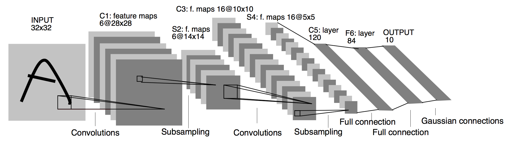
With the rapid development of hardware equipment, deeper neural network layers become. By improving the original convolutional neural network, people have proposed many powerful new models, such as AlexNet, GoogleNet, ResNet, etc. In our project, we are going to apply Residual Network to brick pattern classification and discuss influence of optimizer and hyperparameter to the convergence and accuracy of neural network model.
Ⅱ. Model Selection
Our goal is to train a model that can distinguish five different classes of images: Flemish bond, English bond, Stretcher bond, other patterns and not brick.
Residual Network is currently one of the mainstream models of image processing. It solves the network degradation through the residual structure without increasing the computational complexity. Therefore, it can realize a very deep neural network and extract very rich image features. The classic residual network is mainly divided into ResNet18 series and ResNet50 series. We consider that the number of data sets is large, there are 10000+ samples, and each sample contains three channels of RBG and 200*200 image pixels, so we believe that a relatively deep residual network is needed to complete the image classification task. In addition, to improve the efficiency of high-depth neural network model training, we use the ResNet50 neural network model based on transfer learning. Because the selected ResNet model contains 50 layers and the data set is extremely large, the training time required for the model is also extremely long. To speed up training, we apply transfer learning. Next, the specific information of the two core implementation parts will be introduced, respectively.
A. Structure of ResNet50 Model
The more layers of the network, the more neurons used to extract each level, and the richer the corresponding features that can be extracted. However, if keep increasing the depth of the network, it will cause gradient dispersion or gradient explosion. Although these two can be solved by introducing normalization initialization and intermediate normalization layers, a new problem occurs, network degradation. A specific manifestation of degradation is that as the number of network layers deepens, the accuracy on the training set gradually saturates or even decreases. This problem is not caused by overfitting, so it cannot be avoided through normalization and cross validation.
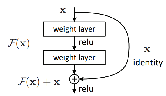
In response to this problem, the developers of ResNet applied the residual block in the new network. The realization of the residual block is also very intuitive: the original input x passes through a conv-relu-conv combination layer, and an F(x) is output, and then this output and the original output are made a sum, namely H(x) =F(x)+x, as shown in the figure above. Therefore, the only difference between the residual block and the original CNN network is that the original input is superimposed on the convolution output through an identity activation function [2]. This branch is called a shortcut.
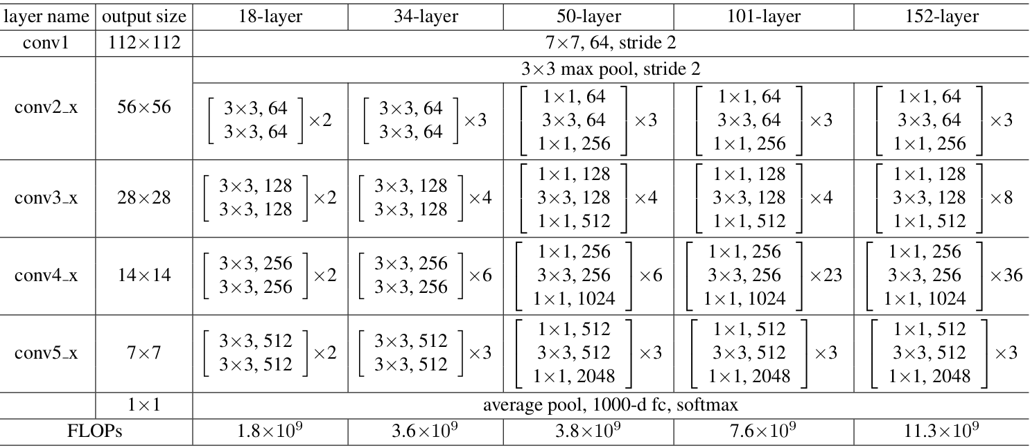
The ResNet50 model used in this experiment is a residual model with a depth of 50 layers obtained by stacking residual blocks, each block contains a 1 × 1, 3 × 3 and another 1 × 1 convolution layer. Construction of the network is shown below.
B. Application of Transfer Learning
Transfer learning is to transfer the parameters of a trained model (pre-trained model on other tasks) to a new model to optimize the training of the new model. Because most of the data and tasks are related, we can transfer the parameters of the pre-training model (which can also be understood as the knowledge learned by the pre-training model) to the new model in some way through migration learning, and then speed up and optimize the learning efficiency of the model.
In this experiment, to accelerate the convergence, we adopted a direct migration method to freeze all the convolutional layers of the original pre-trained model, retain all its parameters, then delete the fully connected layer, and finally add and train this fully-connected layer customized for this task. This experiment needs to train a 5-classes classifier, the original ResNet can recognize 1000 objects. In order to adapt to the data set of this experiment, we replaced the last layer of ResNet and used the input of the original fully connected layer as the input of the new linear layer with 256 output units. Finally, it passes through the ReLu layer and a 256*5 linear layer, and finally outputs a 5-channel softmax. In this way, we can train the specific fully connected layer of this model by directly importing the model parameters of other large-scale data set classification tasks. The advantage of this method is that it can fully retain the image features extracted by the model in other data sets. Such modification of the code can greatly increase the training speed.
C. Improved Model
Transfer learning is to transfer the parameters of a trained model (pre-trained model on other tasks) to a new model to optimize the training of the new model. Because most of the data and tasks are related, we can transfer the parameters of the pre-training model (which can also be understood as the knowledge learned by the pre-training model) to the new model in some way through migration learning, and then speed up and optimize the learning efficiency of the model.
Ⅲ. Experiments Design
In this part, we propose our training strategy, including data preprocessing, optimization algorithm to improve convergence speed, and hyperparameter selection. We also propose solutions to unexpected results that may occur in our test.
A. Experiment Strategy
First of all, we need to prove that transfer learning works in the classification task of brick patterns: we expect that the trained parameters of the convolutional layer in original model are suitable for the image features of the bricks. We only need to train the fully connection layer to obtain model with high accuracy. When comparing model applying or not applying transfer learning, we use same training set and validation set.
After proving that the residual network with transfer learning can finish brick pattern classification, we need to optimize the model. Widely used optimizer include Momentum [3], SGD, and adaptive learning rate algorithms, such as Adagrad and Adam. They can improve convergence speed of training.
Due to the deep network depth, we need a fast convergence and avoid ending with the local optimum. Hence, among the traditional optimization strategies, we choose Momentum. This algorithm considers former batches by introducing momentum to fine-tune the final update direction of the gradient. In this way, the training process can be more stable and faster, and it is possible to jump out from the local optimum. As for the adaptive learning rate algorithm, Adam may not converge, but it is suitable for larger data sets, and the convergence efficiency ranks high in various adaptive learning algorithms. We still chose Adam as the second candidate optimization algorithm.
When looking for better optimization algorithm, we set a series of typical parameters for these two algorithms, including learning rate, momentum and hyperparameters b1, b2, etc. We will use same training set and validation set to train the ResNet50 neural network based on transfer learning each time. After comparing the convergence speed and accuracy under different conditions, we will choose the better combination of optimizer and hyperparameters and save the model for testing.
Finally, we will use the test set to test the generalization ability of the model. If the testing accuracy is lower than that of the validation set, or overfitting occurs obviously, we will increase the scale of training set or adjusting the parameters, such as choosing some atypical values or applying other optimization algorithms which can avoid such problems.
B. Training Flow
In this experiment, a complete model training concludes following main steps:
-
Select model: This experiment uses classic ResNet 50 network model as default module. We download the trained model provided by Pytorch for transfer learning.
-
Divide dataset: We divide the entire dataset and labels into 8:1:1 randomly, the number of training, validation and testing samples are 9106, 1138 and 1139, respectively.
-
Data preprocessing: Preprocessing mainly includes two parts. First, in the pre-training model used for transfer learning, the size of input image is 2242243 channels. To match it well, we use bilinear interpolation to resize the pixels of given images from 200200 to 224224. Compared with the zero-filling method, interpolation can preserve the features of the image. Second, we need to normalize each channel, which can speed up the convergence and avoid numerical overflow
-
Set Batch size: Smaller batch size requires more iterations, which means that each epoch needs long time to finish training and may not converge; Large batch size occupies large memory of GPU and the model may drop into saddle point. Considering the trade-off of time and space, we conclude that for a data set with 10000 samples, it is a good choice to set batch size to 32, which is also the maximum value that our laptops allow.
-
Select optimizer and parameters: For the Momentum optimizer, the typical learning rate is [0,001, 0.001, 0.1] and the hyperparameter is momentum, which is 0.9 as default. For the adaptive learning rate optimizer Adam, the typical initial learning rate is [1e-4, 0.001, 0.01] and the hyperparameter is b1 and b2, which is 0.9 and 0.99, respectively.
-
Set max epoch as 30 and start training. In each epoch, we calculate the average loss and the accuracy of validation set. We save the parameters of model with highest accuracy rate among all epochs.
-
Save the training record after 30 epochs as .npy file, which includes the loss and the accuracy of each epoch. Then the training is finished.
C. Testing Flow
After importing the testing set, they need to be preprocessed in the same way to the training set, that is, size transformation and normalization. Besides, the batch size is also 32. We will load the best Residual network model for training and show confusion matrix and accuracy.
If the test accuracy is much lower than results of validation set, we will re-select the optimizer or use the residual network with shallower network layers, such as ResNet18, because the model with lower complexity is less prone to overfitting.
Ⅳ. Result and Analysis
Experiment 1: Prove the parameters of convolution layers of trained model is effective in the brick pattern classification.
We use ResNet50 model; divide the dataset randomly, 80% is training set and 10% is validation set; the optimizer is Adam, with hyperparameter b1 and b2, which is 0.9 and 0.99. We test two times with different initial learning rate, 0.01 and 0.001. Here gives the loss curves of using/ not using transfer learning.
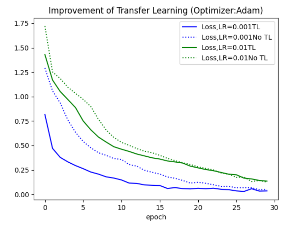
The trend of the solid lines and the dashed lines in this picture is same, which proves that the trained convolutional layer parameters we used are suitable for brick pattern recognition. We also found that using the same training set for training, transfer learning cannot significantly improve the convergence rate, and the loss rate is the same for larger epochs to the result of non-transfer learning. But transfer learning can significantly reduce the initial loss, so that the neural network reaches the optimum point faster and improves the training efficiency.
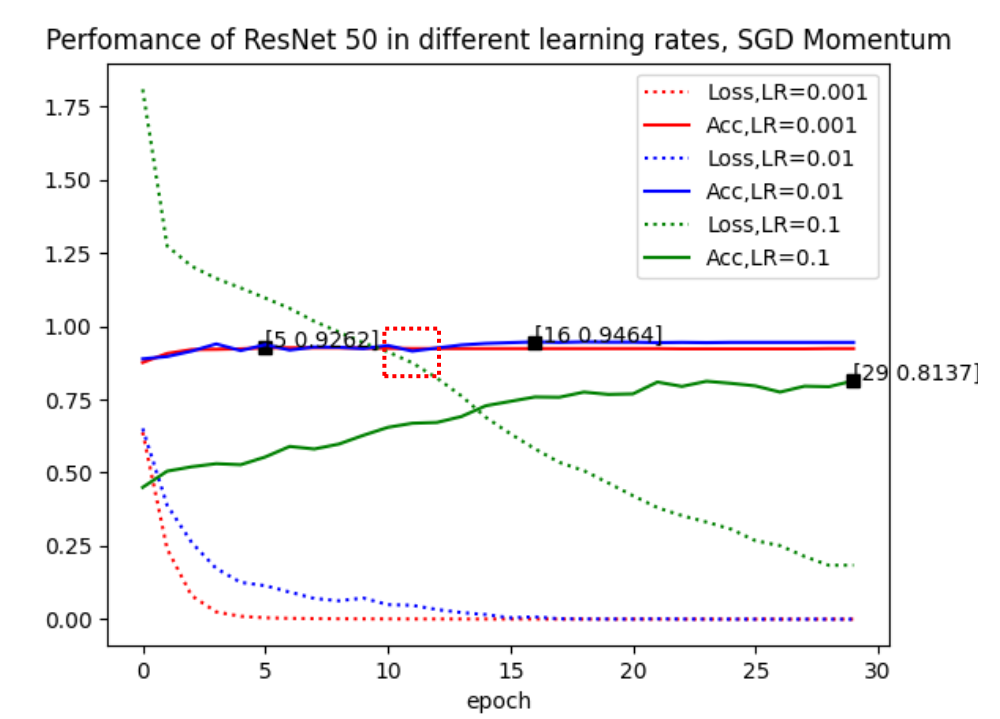
We chose same model and hyperparameters as Experiment 1 and compare the convergence under typical values of learning rates for different optimizer, Adam and Momentum. The test results are shown in Figure 2 and Figure 3, respectively.
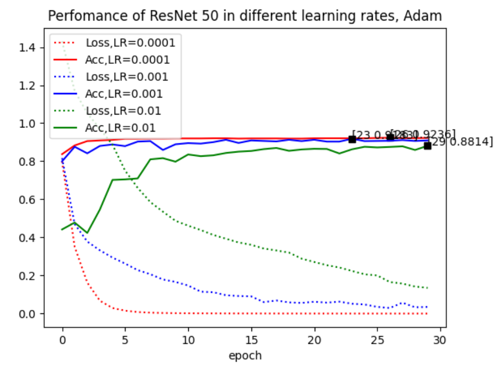
The results show that Momentum optimizer is more suitable for our classification task than Adam. We also found that the accuracy rate is not proportional to the speed of convergence. When adjusting the parameter of Momentum, the model with learning rate of 0.001 achieve the best accuracy of 92.6% in the 5th epoch, but when learning rate is changed to 0.01, although the convergence becomes slower, finding optimum at the 16th epoch, the accuracy rate reaches as high as 94.6%, which is better than the former setting. It indicates that the model has gone into a better optimum point at this learning rate.
Therefore, we will use Momentum optimizer with a learning rate of 0.01 in the future test.
Experiment 3: Apply our trained ResNet 50 model to the blind testing set with 1139 samples.
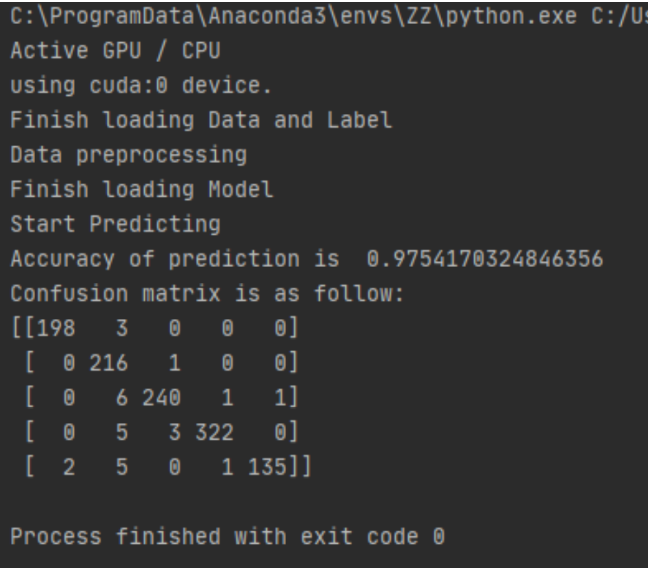
The test result is surprising! The accuracy rate of blind test set is 97.5%, much higher to the verification set. It shows that there is not over-fitting in our model and this ResNet50 model looks perfect.
Ⅴ. Conclusion
Deeper neural networks may become a trend in the future, and the residual networks makes efficient training of such deep networks possible. Our experiment gives the reasons for the selection of model, optimization algorithm, and parameter, and we obtained a very good model by analyzing and comparing a large number of training results.
In our experiments, we found that transfer learning can significantly reduce the initial loss, which greatly reduces the times of epoch needed to obtain the extremum. The choice of optimizer and learning rate will also significantly impact the accuracy of the model. In detail, in the task of brick pattern recognition, the Momentum algorithm can obtain a verification accuracy of 94.5% at a learning rate of 0.01, which performs better than Adam of 92.3%. This is because the introduction of momentum makes the model more likely to jump out of the local optimum and find the global optimum.
Our experiment did not research on the depth of the residual network and the influence of the value of momentum to the task of brick pattern recognition. We think it is worth to do more on it. We also look forward to studying the performance of this model in classification tasks with more categories.
In general, under the application of migration learning and Momentum optimization algorithm, the ResNet50 model can make the network converge to the extreme value with fewer epochs <15, and the correct rate of the verification set is always above 90%. This is a very efficient training method. Our test results are also very satisfactory, with an accuracy rate of 97.5% on the blind test set. We are confident that our model can have good performance in other test sets.
References
[1] Y. Yang, J. Wang and Y. Yang, “Improving SVM classifier with prior knowledge in microcalcification detection1,” 2012 19th IEEE International Conference on Image Processing, Orlando, FL, 2012, pp. 2837-2840.
[2] A. Budhiman, S. Suyanto and A. Arifianto, “Melanoma Cancer Classification Using ResNet with Data Augmentation,” 2019 International Seminar on Research of Information Technology and Intelligent Systems (ISRITI), Yogyakarta, Indonesia, 2019, pp. 17-20.
[3] A. Srivastava and H. R. Arabnia, “Asynchronous Variance Reduced SGD with Momentum Tuning in Edge Computing,” 2018 International Conference on Computational Science and Computational Intelligence (CSCI), Las Vegas, NV, USA, 2018, pp. 1059-1064.
[4] Z. Zhang, “Improved Adam Optimizer for Deep Neural Networks,” 2018 IEEE/ACM 26th International Symposium on Quality of Service (IWQoS), Banff, AB, Canada, 2018, pp. 1-2.
Click here to view code for this project